ancient_trichuris

Principle component analysis to explore genetic diversity

Author: Stephen Doyle, stephen.doyle[at]sanger.ac.uk

PCA of mitochondrial variants
PCA of nuclear variants

PCA of mitochondrial variation

# working directory
/nfs/users/nfs_s/sd21/lustre118_link/trichuris_trichiura/05_ANALYSIS/PCA

# load libraries
library(tidyverse)
library(gdsfmt)
library(SNPRelate)
library(ggsci)

snpgdsClose(genofile)

vcf.in <- "mito_samples3x_missing0.8.recode.vcf.gz"

gds <- snpgdsVCF2GDS(vcf.in, "mtDNA_1.gds", method="biallelic.only")

genofile <- snpgdsOpen(gds)

pca <- snpgdsPCA(genofile, num.thread=2, autosome.only = F)

samples <- as.data.frame(pca$sample.id)

colnames(samples) <- "name"

metadata <- samples %>% separate(name,c("time", "country","population","host","sampleID"))

metadata <- metadata %>%
  mutate(SAMPLE_AGE = ifelse(time == "AN", "Ancient",
               ifelse(host == "HS", "Modern Human", "Modern Animal")))


data <-
     data.frame(sample.id = pca$sample.id,
          EV1 = pca$eigenvect[,1],
          EV2 = pca$eigenvect[,2],
          EV3 = pca$eigenvect[,3],
          EV4 = pca$eigenvect[,4],
          EV5 = pca$eigenvect[,5],
          EV6 = pca$eigenvect[,6],
          TIME = metadata$SAMPLE_AGE,
          COUNTRY = metadata$country,
          POPULATION = metadata$population,
          HOST = metadata$host,
          stringsAsFactors = FALSE)

country_colours <-
     c("CHN" = "#00A087",
     "CMR" = "#902F21",
     "DNK" = "#3C5488",
     "ESP" = "#E7EAF0",
     "HND" = "#4DBBD5",
     "NLD" = "#9DAAC4",
     "UGA" = "#E64B35",
     "LTU" = "#0F1522",
     "TZA" = "#F2A59A")


plot_pca <-
     ggplot(data, aes(EV1, EV2, col = COUNTRY, shape = TIME, label = COUNTRY)) +
     geom_text(size=4) +
     theme_bw() +
     labs(title="mito_samples3x_missing0.8",
          x = paste0("PC1 variance: ",round(pca$varprop[1]*100,digits=2),"%"),
          y = paste0("PC2 variance: ",round(pca$varprop[2]*100,digits=2),"%"))+
     scale_colour_manual(values = country_colours)

plot_pca

ggsave("plot_PCA_mito_samples3x_missing0.8.png")

# use this to label with sample names
#ggplot(tab,aes(EV1,EV2, col = COUNTRY, shape = TIME, label = COUNTRY)) + geom_point(size=4)

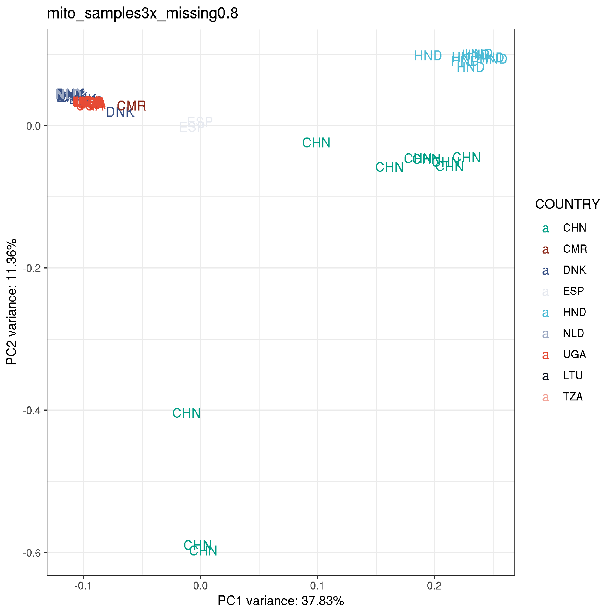
the CHN LF samples are the outliers in the above plot, so rerunning to remove these

vcftools \
--gzvcf Trichuris_trichiura.cohort.mito_variants.final.recode.vcf.gz \
--keep mtDNA_3x_noLF.list \
--max-missing 0.8 \
--recode --recode-INFO-all \
--out mito_samples3x_missing0.8_noLF

gzip -f mito_samples3x_missing0.8_noLF*

#> After filtering, kept 48 out of 61 Individuals
#> After filtering, kept 1291 out of a possible 1888 Sites

# load libraries
library(tidyverse)
library(gdsfmt)
library(SNPRelate)
library(ggsci)
library(patchwork)

snpgdsClose(genofile)
vcf.in <- "mito_samples3x_missing0.8_noLF.recode.vcf.gz"
gds <- snpgdsVCF2GDS(vcf.in, "mtDNA.gds", method="biallelic.only")

genofile <- snpgdsOpen(gds)

pca <- snpgdsPCA(genofile, num.thread=2, autosome.only = F)
# Working space: 56 samples, 802 SNPs

samples <- as.data.frame(pca$sample.id)
colnames(samples) <- "name"

metadata <- samples %>% separate(name,c("time", "country","population","host","sampleID"))
metadata <- metadata %>%
  mutate(SAMPLE_AGE = ifelse(time == "AN", "Ancient",
               ifelse(host == "HS", "Modern Human", "Modern Animal")))


data <-
     data.frame(sample.id = pca$sample.id,
          EV1 = pca$eigenvect[,1],
          EV2 = pca$eigenvect[,2],
          EV3 = pca$eigenvect[,3],
          EV4 = pca$eigenvect[,4],
          EV5 = pca$eigenvect[,5],
          EV6 = pca$eigenvect[,6],
          TIME = metadata$SAMPLE_AGE,
          COUNTRY = metadata$country,
          POPULATION = metadata$population,
          HOST = metadata$host,
          stringsAsFactors = FALSE)

country_colours <-
     c("CHN" = "#00A087",
     "CMR" = "#902F21",
     "DNK" = "#3C5488",
     "ESP" = "#E7EAF0",
     "HND" = "#4DBBD5",
     "NLD" = "#9DAAC4",
     "UGA" = "#E64B35",
     "LTU" = "#0F1522",
     "TZA" = "#F2A59A")


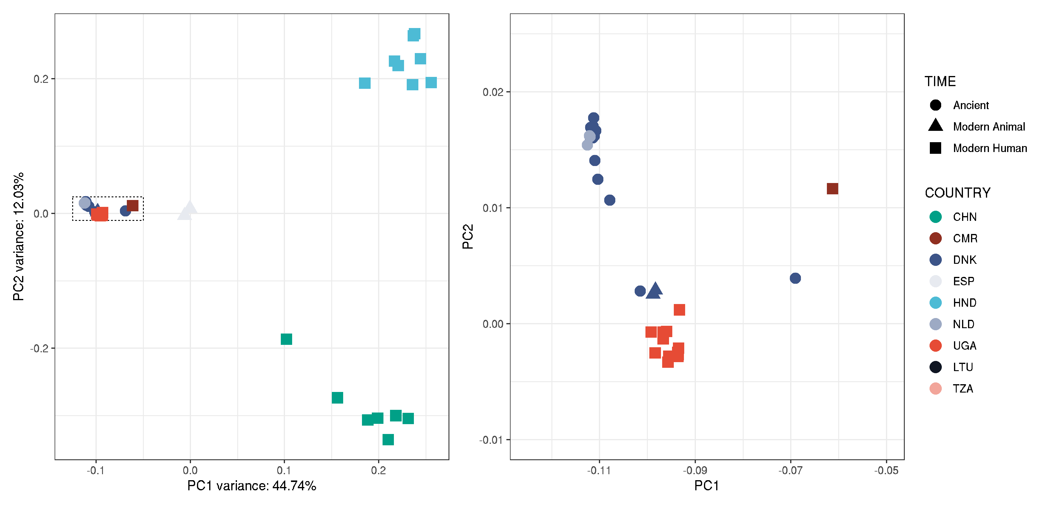
plot_pca_mito <-
     ggplot(data, aes(EV1, EV2, col = COUNTRY, shape = TIME, label = COUNTRY),alpha=1) +
     geom_rect(aes(xmin=-0.125, ymin=-0.01, xmax=-0.05, ymax=0.025), fill=NA, col="black", linetype="dotted", size=0.3) +
     geom_point(size=4, alpha=1) +
     theme_bw() +
     labs(x = paste0("PC1 variance: ",round(pca$varprop[1]*100,digits=2),"%"),
          y = paste0("PC2 variance: ",round(pca$varprop[2]*100,digits=2),"%")) +
     scale_colour_manual(values = country_colours)

plot_pca_mito_zoom <-
     ggplot(data, aes(EV1,EV2, col = COUNTRY, shape = TIME, label = paste0(TIME,"_",COUNTRY,"_",POPULATION,"_",HOST))) +
     geom_point(size=4, alpha=1) +
     theme_bw() +
     labs(x = "PC1",
          y = "PC2") +
     xlim(-0.125,-0.05) + ylim(-0.01, 0.025) +
     scale_colour_manual(values = country_colours)

# note: geom_rect in first plot and zoom coordinates were adjusted manually to show the cluster clearly.


plot_pca_mito + plot_pca_mito_zoom + plot_layout(ncol=2, guides = "collect")

ggsave("plot_PCA_mito_samples3x_missing0.8_noLF.png")
ggsave("plot_PCA_mito_samples3x_missing0.8_noLF.pdf", height = 5, width = 11, useDingbats=FALSE)

Figure: plot_PCA_mito_samples3x_missing0.8_noLF

will uses this in Figure 1 panels A and B

PCA of nuclear variants

human + animal + 2 ancients
“nuclear_3x_animal.list”

# extract nuclear variants

# vcftools \
# --gzvcf Trichuris_trichiura.cohort.nuclear_variants.final.recode.vcf.gz \
# --keep nuclear_3x_animal.list \
# --max-missing 0.8 \
# --recode --recode-INFO-all \
# --out nuclear_samples3x_missing0.8

# post peer review - restricted to autosomes only, excluding sex chromosomes
vcftools \
--gzvcf Trichuris_trichiura.cohort.nuclear_variants.final.recode.vcf.gz \
--keep nuclear_3x_animal.list \
--max-missing 0.8 \
--recode --recode-INFO-all \
--bed trichuris_trichiura.autosomeLG.bed \
--out nuclear_samples3x_missing0.8

gzip -f nuclear_samples3x_missing0.8.recode.vcf

#> After filtering, kept 36 out of 61 Individuals
#> After filtering, kept 1850621 out of a possible 6933531 Sites

# load libraries
library(tidyverse)
library(gdsfmt)
library(SNPRelate)
library(patchwork)

snpgdsClose(genofile)

vcf.in <- "nuclear_samples3x_missing0.8.recode.vcf.gz"

gds<-snpgdsVCF2GDS(vcf.in, "nuclear_1.gds", method="biallelic.only")

genofile <- snpgdsOpen(gds)

pca <- snpgdsPCA(genofile, num.thread=2, autosome.only = F)
# Working space: 36 samples, 1,675,392 SNPs

samples <- as.data.frame(pca$sample.id)

colnames(samples) <- "name"

metadata <- samples %>% separate(name,c("time", "country","population","host","sampleID"))
metadata <- metadata %>%
  mutate(SAMPLE_AGE = ifelse(time == "AN", "Ancient",
               ifelse(host == "HS", "Modern Human", "Modern Animal")))


data <-
     data.frame(sample.id = pca$sample.id,
          EV1 = pca$eigenvect[,1],
          EV2 = pca$eigenvect[,2],
          EV3 = pca$eigenvect[,3],
          EV4 = pca$eigenvect[,4],
          EV5 = pca$eigenvect[,5],
          EV6 = pca$eigenvect[,6],
          TIME = metadata$SAMPLE_AGE,
          COUNTRY = metadata$country,
          POPULATION = metadata$population,
          HOST = metadata$host,
          stringsAsFactors = FALSE)

country_colours <-
     c("CHN" = "#00A087",
     "CMR" = "#902F21",
     "DNK" = "#3C5488",
     "ESP" = "#E7EAF0",
     "HND" = "#4DBBD5",
     "NLD" = "#9DAAC4",
     "UGA" = "#E64B35",
     "LTU" = "#0F1522",
     "TZA" = "#F2A59A")

plot_pca_nuc <-
     ggplot(data,aes(EV1, EV2, col = COUNTRY, shape = TIME, label = HOST)) +
     geom_point(size=4) +
     geom_text_repel(size=4) +
     theme_bw() +
     labs(title="nuclear_samples3x_missing0.8",
          x = paste0("PC1 variance: ",round(pca$varprop[1]*100,digits=2),"%"),
          y = paste0("PC2 variance: ",round(pca$varprop[2]*100,digits=2),"%"))+
     scale_colour_manual(values = country_colours)

plot_pca_nuc

ggsave("plot_PCA_nuclear_samples3x_missing0.8.png")
ggsave("plot_PCA_nuclear_samples3x_missing0.8.pdf", height=5, width=5)

main outliers are colobus and leafmonkey, so will remove and rerun

# vcftools \
# --gzvcf Trichuris_trichiura.cohort.nuclear_variants.final.recode.vcf.gz \
# --keep nuclear_3x_animalPhonly.list \
# --max-missing 0.8 \
# --recode --recode-INFO-all \
# --out nuclear_samples3x_missing0.8_animalPhonly

# post peer review - restricted to autosomes only, excluding sex chromosomes
vcftools \
--gzvcf Trichuris_trichiura.cohort.nuclear_variants.final.recode.vcf.gz \
--keep nuclear_3x_animalPhonly.list \
--max-missing 0.8 \
--recode --recode-INFO-all \
--bed trichuris_trichiura.autosomeLG.bed \
--out nuclear_samples3x_missing0.8_animalPhonly

gzip -f nuclear_samples3x_missing0.8_animalPhonly.recode.vcf

#> After filtering, kept 31 out of 61 Individuals
#> After filtering, kept 1963868 out of a possible 6933531 Sites

# load libraries
library(tidyverse)
library(gdsfmt)
library(SNPRelate)
library(ggsci)

snpgdsClose(genofile)

vcf.in <- "nuclear_samples3x_missing0.8_animalPhonly.recode.vcf.gz"

gds <- snpgdsVCF2GDS(vcf.in, "nuclear.gds", method="biallelic.only")

genofile <- snpgdsOpen(gds)

pca <- snpgdsPCA(genofile, num.thread=2, autosome.only = F)
# Working space: 31 samples, 2,544,110 SNPs

samples <- as.data.frame(pca$sample.id)

colnames(samples) <- "name"

metadata <- samples %>% separate(name,c("time", "country","population","host","sampleID"))

# fix the metadata so can get the right shapes to match the main sampling map
metadata <- metadata %>%
  mutate(SAMPLE_AGE = ifelse(time == "AN", "Ancient",
               ifelse(host == "HS", "Modern Human", "Modern Animal")))


data <-
     data.frame(sample.id = pca$sample.id,
          EV1 = pca$eigenvect[,1],
          EV2 = pca$eigenvect[,2],
          EV3 = pca$eigenvect[,3],
          EV4 = pca$eigenvect[,4],
          EV5 = pca$eigenvect[,5],
          EV6 = pca$eigenvect[,6],
          TIME = metadata$SAMPLE_AGE,
          COUNTRY = metadata$country,
          POPULATION = metadata$population,
          HOST = metadata$host,
          stringsAsFactors = FALSE)

country_colours <-
     c("CHN" = "#00A087",
     "CMR" = "#902F21",
     "DNK" = "#3C5488",
     "ESP" = "#E7EAF0",
     "HND" = "#4DBBD5",
     "NLD" = "#9DAAC4",
     "UGA" = "#E64B35",
     "LTU" = "#0F1522",
     "TZA" = "#F2A59A")



plot_pca_nuc <-
     ggplot(data,aes(EV1, EV2, col = COUNTRY, shape = TIME)) +
     geom_point(size=4, alpha=1) +
     theme_bw() +
     labs(x = paste0("PC1 variance: ",round(pca$varprop[1]*100,digits=2),"%"),
          y = paste0("PC2 variance: ",round(pca$varprop[2]*100,digits=2),"%")) +
     scale_colour_manual(values = country_colours)

plot_pca_nuc_labels <-
     ggplot(data,aes(EV1, EV2, col = COUNTRY, shape = TIME, label = POPULATION)) +
     geom_point(size=4, alpha=1) +
     geom_text_repel() +
     theme_bw() +
     labs(x = paste0("PC1 variance: ",round(pca$varprop[1]*100,digits=2),"%"),
          y = paste0("PC2 variance: ",round(pca$varprop[2]*100,digits=2),"%")) +
     scale_colour_manual(values = country_colours)

plot_pca_nuc

# plot
ggsave("plot_PCA_nuclear_samples3x_missing0.8_animalPhonly.pdf", height = 5, width = 5, useDingbats=FALSE)
ggsave("plot_PCA_nuclear_samples3x_missing0.8_animalPhonly.png")




plot_pca_mito + plot_pca_mito_zoom + plot_pca_nuc + plot_layout(ncol=3, guides = "collect")

ggsave("plot_PCA_mito_mitozoom_nuc.pdf", height = 4, width = 14, useDingbats=FALSE)
ggsave("plot_PCA_plot_PCA_mito_mitozoom_nuc.png")

Figure: plot_PCA_nuclear_samples3x_missing0.8_animalPhonly

to be used in Figure 1, panel D

ancient_trichuris

Principle component analysis to explore genetic diversity

Contents

PCA of mitochondrial variation

PCA of nuclear variants