ancient_trichuris

Genome-wide genetic variation

Author: Stephen Doyle, stephen.doyle[at]sanger.ac.uk

Contents

• Running pixy to calculate nucleotide diversity, dXY and Fst between groups
• analyses of nucleotide diversity (Pi)
• dXY and Fst
• extracting top X% of Fst values for each comparison
• Private and shared variation between populations
• Ancient DNA - nucleotide diversity vs sampling age
• Sample Heterozygosity vs sequencing coverage
• Relatedness and kinship between samples in a population
• genome-wide analyses presented in the original draft of the manuscript, but subsequently improved upon

Running pixy to calculate nucleotide diversity, dXY and Fst between groups

conda activate pixy

cp ../../04_VARIANTS/GATK_HC_MERGED/nuclear_samples3x_missing0.8_animalPhonly.recode.vcf.gz .

gunzip nuclear_samples3x_missing0.8_animalPhonly.recode.vcf.gz
bgzip nuclear_samples3x_missing0.8_animalPhonly.recode.vcf
tabix -p vcf nuclear_samples3x_missing0.8_animalPhonly.recode.vcf.gz

bsub.py --queue yesterday --threads 2 10 pixy \
"pixy --stats pi fst dxy \
     --vcf nuclear_samples3x_missing0.8_animalPhonly.recode.vcf.gz \
     --populations populations.list \
     --window_size 20000 \
     --bypass_invariant_check 'yes' \
     --n_cores 2"

# using a vcf with all sites
bsub.py --queue long --threads 20 20 pizy_allsites \
"pixy --stats pi fst dxy \
--vcf Trichuris_trichiura.cohort.allsites.vcf.gz \
--populations populations.list \
--window_size 20000 \
--n_cores 20 \
--output_prefix trichuris_allsites"

analyses of nucleotide diversity (Pi)

# load libraries
library(tidyverse)
library(patchwork)
library(ggridges)

# get nucleotide diversity (pi) data from pixy output
pi_data <- read.table("trichuris_allsites_pi.txt", header=T)


# subset
pi_data_an <- pi_data %>%
     filter(pop=="AN" & !str_detect(chromosome, "^Trichuris_trichiura_00"))
pi_data_HND <- pi_data %>%
     filter(pop=="HND" & !str_detect(chromosome, "^Trichuris_trichiura_00"))
pi_data_CHN <- pi_data %>%
     filter(pop=="CHN" & !str_detect(chromosome, "^Trichuris_trichiura_00"))

# filter pi data to remove small scaffolds not in the linkage groups, and to number the rows per group to help with plotting
pi_data <- pi_data %>%
     filter(!str_detect(chromosome, "^Trichuris_trichiura_00")) %>%
     group_by(pop) %>%
     mutate(position = 1:n())


# get position for vertical lines used in plot to delineate the linkage groups
pi_data %>%
     group_by(chromosome) %>%
     summarise(max = max(position, na.rm = TRUE))

     # A tibble: 19 × 2
        /* chromosome                  max
        <chr>                     <int>
      1 Trichuris_trichiura_1_001   565
      2 Trichuris_trichiura_1_002   821
      3 Trichuris_trichiura_1_003   922
      4 Trichuris_trichiura_1_004   996
      5 Trichuris_trichiura_1_005  1057
      6 Trichuris_trichiura_1_006  1099
      7 Trichuris_trichiura_1_007  1125 <<
      8 Trichuris_trichiura_2_001  2584 <<
      9 Trichuris_trichiura_3_001  3043
     10 Trichuris_trichiura_3_002  3321
     11 Trichuris_trichiura_3_003  3453
     12 Trichuris_trichiura_3_004  3512
     13 Trichuris_trichiura_3_005  3547
     14 Trichuris_trichiura_3_006  3574
     15 Trichuris_trichiura_3_007  3592
     16 Trichuris_trichiura_3_008  3608
     17 Trichuris_trichiura_3_009  3620
     18 Trichuris_trichiura_3_010  3628
     19 Trichuris_trichiura_MITO   3629 */


pi_data <- pi_data %>%
     mutate(chr_type = ifelse(str_detect(chromosome, "^Trichuris_trichiura_1"), "sexchr", "autosome"))


# calculate the median Pi and checking the ratio of sex-to-autosome diversity. Should be about 0.75, as Trichuris is XX/XY
pi_data_sex_median <- pi_data %>%
     group_by(chr_type) %>%
     summarise(median = median(avg_pi, na.rm = TRUE))

#     # A tibble: 2 × 2
#       chr_type  median
#       <chr>      <dbl>
#     1 autosome 0.00849
#     2 sexchr   0.00610

# 0.00610 / 0.00849 = 0.72 (not far off 0.75 expected of diversity on sex chromosome relative to autosome)

pi_data_pop-sex_median <- pi_data %>%
     group_by(pop, chr_type) %>%
     summarise(median = median(avg_pi, na.rm = TRUE))

     # # A tibble: 10 × 3
     # # Groups:   pop [5]
     #    pop    chr_type  median
     #    <chr>  <chr>      <dbl>
     #  1 AN     autosome 0.00432
     #  2 AN     sexchr   0.00236
     #  3 BABOON autosome 0.0111
     #  4 BABOON sexchr   0.00562
     #  5 CHN    autosome 0.0112
     #  6 CHN    sexchr   0.00849
     #  7 HND    autosome 0.00871
     #  8 HND    sexchr   0.00643
     #  9 UGA    autosome 0.0128
     # 10 UGA    sexchr   0.0102



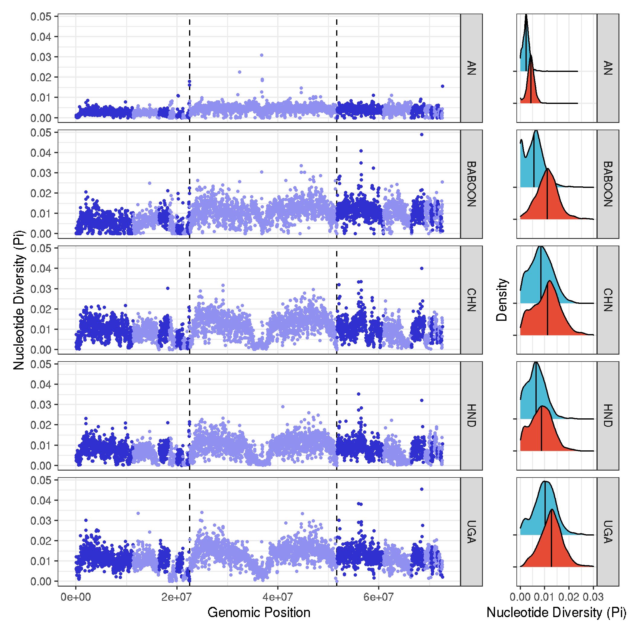
# plot 1 - genome wide plots per population
plot_1 <- ggplot(pi_data, aes(position*20000, avg_pi, col=chromosome)) +
     geom_vline(xintercept=c(1125*20000,2584*20000),size=0.5, linetype="dashed")+
     geom_point(size=0.5) +
     facet_grid(pop~.) +
     scale_colour_cyclical(values = c("#3030D0", "#9090F0")) +
     theme_bw() +
     labs(x="Genomic Position", y="Nucleotide Diversity (Pi)")


# plot 2 - density plots of pi per group
plot_2 <- ggplot(pi_data, aes(avg_pi, chr_type, fill=chr_type), guide="none") +
     geom_density_ridges(quantile_lines=TRUE, quantile_fun=function(x,...)median(x), size=0.5) +
     theme_bw() + theme(legend.position = "none", axis.text.y=element_blank()) +
     facet_grid(pop~.) +
     xlim(0,0.03) +
     scale_fill_npg() +
     labs(x="Nucleotide Diversity (Pi)", y="Density")

# bring it together
plot_1 + plot_2 +  plot_layout(widths = c(5, 1))

ggsave("plots_genomewide_and_density_Pi.pdf", width=7, height=6, useDingbats=FALSE)
ggsave("plots_genomewide_and_density_Pi.png")

dXY and Fst

• need to recreate datasets showing dXY and Fst for
  • CHN vs UGA
  • HND vs UGA
  • CHN vs HND
  • BABOON vs UGA

# load libraries
library(tidyverse)
library(ggridges)

# load data
dxy_data <- read.table("trichuris_allsites_dxy.txt", header=T)
fst_data <- read.table("trichuris_allsites_fst.txt", header=T)

# add some columns
dxy_data$data_type <- "Dxy"
dxy_data <- mutate(dxy_data,
     comparison = paste(pop1, pop2, sep = '_v_'))

fst_data$data_type <- "Fst"
fst_data <- mutate(fst_data,
     comparison = paste(pop1, pop2, sep = '_v_'))

# subset and merge dataframes
dxy_data_sub <- dxy_data %>% select(comparison,data_type,chromosome,window_pos_1,window_pos_2,avg_dxy)
colnames(dxy_data_sub) <- c("comparison","data_type","chromosome","window_pos_1","window_pos_2","value")

fst_data_sub <- fst_data %>% select(comparison,data_type,chromosome,window_pos_1,window_pos_2,avg_wc_fst)
colnames(fst_data_sub) <- c("comparison","data_type","chromosome","window_pos_1","window_pos_2","value")

# cheeky fix to get matching rows from both datasets
tmp_dxy <- semi_join(dxy_data_sub, fst_data_sub, by=c("comparison", "chromosome", "window_pos_1", "window_pos_2"))
tmp_fst <- semi_join(fst_data_sub, dxy_data_sub,  by=c("comparison", "chromosome", "window_pos_1", "window_pos_2"))

# join the datasets together to create a single dataframe
data <- full_join(tmp_dxy, tmp_fst)

# add numbering to help with plotting
data <- data %>%
     filter(!str_detect(chromosome, "^Trichuris_trichiura_00")) %>%
     group_by(comparison, data_type) %>%
     mutate(position = 1:n())

# add sex chromosome information
data <- data %>%
     mutate(chr_type = ifelse(str_detect(chromosome, "^Trichuris_trichiura_1"), "sexchr", "autosome"))

# get position for vertical lines used in plot to delineate the linkage groups
data %>%
     group_by(chromosome) %>%
     summarise(max = max(position, na.rm = TRUE))

     # # A tibble: 19 × 2
     #    chromosome                  max
     #    <chr>                     <int>
     #  1 Trichuris_trichiura_1_001   565
     #  2 Trichuris_trichiura_1_002   820
     #  3 Trichuris_trichiura_1_003   921
     #  4 Trichuris_trichiura_1_004   994
     #  5 Trichuris_trichiura_1_005  1055
     #  6 Trichuris_trichiura_1_006  1097
     #  7 Trichuris_trichiura_1_007  1122 <<<
     #  8 Trichuris_trichiura_2_001  2580 <<<
     #  9 Trichuris_trichiura_3_001  3038
     # 10 Trichuris_trichiura_3_002  3316
     # 11 Trichuris_trichiura_3_003  3448
     # 12 Trichuris_trichiura_3_004  3507
     # 13 Trichuris_trichiura_3_005  3542
     # 14 Trichuris_trichiura_3_006  3569
     # 15 Trichuris_trichiura_3_007  3586
     # 16 Trichuris_trichiura_3_008  3602
     # 17 Trichuris_trichiura_3_009  3614
     # 18 Trichuris_trichiura_3_010  3622
     # 19 Trichuris_trichiura_MITO   3623

# summarise median data for Fst and Dxy
data %>%
     group_by(comparison,data_type) %>%
     summarise(median = median(value, na.rm = TRUE))

     # # Groups:   comparison [10]
     #    comparison   data_type  median
     #    <chr>        <chr>       <dbl>
     #  1 AN_v_BABOON  Dxy       0.00761
     #  2 AN_v_BABOON  Fst       0.0259
     #  3 AN_v_CHN     Dxy       0.0112
     #  4 AN_v_CHN     Fst       0.238
     #  5 AN_v_HND     Dxy       0.0118
     #  6 AN_v_HND     Fst       0.375
     #  7 AN_v_UGA     Dxy       0.00951
     #  8 AN_v_UGA     Fst       0.0662
     #  9 BABOON_v_CHN Dxy       0.0153
     # 10 BABOON_v_CHN Fst       0.298
     # 11 BABOON_v_HND Dxy       0.0158
     # 12 BABOON_v_HND Fst       0.414
     # 13 BABOON_v_UGA Dxy       0.0136
     # 14 BABOON_v_UGA Fst       0.148
     # 15 HND_v_CHN    Dxy       0.0133
     # 16 HND_v_CHN    Fst       0.269
     # 17 HND_v_UGA    Dxy       0.0146
     # 18 HND_v_UGA    Fst       0.279
     # 19 UGA_v_CHN    Dxy       0.0131
     # 20 UGA_v_CHN    Fst       0.116


# plotted Fst and Dxy together, but it is very noisy.
# #subset by comparison
# data_CHNvUGA <- data %>% filter(comparison=="UGA_v_CHN")
# data_HNDvUGA <- data %>% filter(comparison=="HND_v_UGA")
# data_HNDvCHN <- data %>% filter(comparison=="HND_v_CHN")
# data_BABOONvUGA <- data %>% filter(comparison=="BABOON_v_UGA")
#
#
# # plot
# plot_fst_dxy <- function(data){
#      ggplot(data, aes(position*20000, value, col=chromosome)) +
#      geom_point(size=0.5) +
#      scale_colour_cyclical(values = c("#3030D0", "#9090F0")) +
#      geom_vline(xintercept=c(1083*20000,2520*20000))+
#      facet_grid(data_type~comparison) +
#      ylim(0,1) +
#      theme_bw() +
#      labs(x="Genomic Position", y="Genetic differentiation")
# }
#
# plot_CHNvUGA <- plot_fst_dxy(data_CHNvUGA)
# plot_HNDvUGA <- plot_fst_dxy(data_HNDvUGA)
# plot_HNDvCHN <- plot_fst_dxy(data_HNDvCHN)
# plot_BABOONvUGA <- plot_fst_dxy(data_BABOONvUGA)
#
# plot_CHNvUGA + plot_HNDvUGA + plot_HNDvCHN + plot_BABOONvUGA + plot_layout(ncol=1)

# # subset data to get only fst values
# data_fst <- data %>% filter(data_type=="Fst" & (comparison=="UGA_v_CHN" | comparison=="HND_v_UGA" | comparison=="HND_v_CHN" | comparison=="BABOON_v_UGA"))
#
# # median values for density plots
# data_fst_median <- data_fst %>%
#      group_by(comparison) %>%
#      summarise(median = median(value, na.rm = TRUE))
#
# # genomewide plot of fst values for each pairwise comparison
# plot_fst_gw <- ggplot(data_fst, aes(position*20000, value, col=chromosome)) +
#      geom_vline(xintercept=c(1083*20000,2520*20000),size=0.5)+
#       geom_point(size=0.5) +
#       scale_colour_cyclical(values = c("#3030D0", "#9090F0")) +
#       facet_grid(comparison~.) +
#       ylim(0,1) +
#       theme_bw() +
#       labs(x="Genomic Position", y="Genetic differentiation")
#
# plot_fst_density <- ggplot(data_fst, aes(value, col=comparison, fill=comparison)) +
#      geom_density(show.legend = FALSE) +
#      facet_grid(comparison~.) +
#      theme_bw() + xlim(0,1) +
#      geom_vline(data=data_fst_median,aes(xintercept=median),linetype="dashed")+
#      labs(x="Genetic differentiation (Fst)", y="Density") +
#      theme()
#
# plot_fst_gw + plot_fst_density +  plot_layout(widths = c(5, 1))
#
#
# # dxy data
# # subset data to get only dxy values
# data_dxy <- data %>% filter(data_type=="Dxy" & (comparison=="UGA_v_CHN" | comparison=="HND_v_UGA" | comparison=="HND_v_CHN" | comparison=="BABOON_v_UGA"))
#
# # median values for density plots
# data_dxy_median <- data_dxy %>%
#      group_by(comparison) %>%
#      summarise(median = median(value, na.rm = TRUE))
#
# # genomewide plot of dxy values for each pairwise comparison
# plot_dxy_gw <- ggplot(data_dxy, aes(position*20000, value, col=chromosome)) +
#      geom_vline(xintercept=c(1083*20000,2520*20000),size=0.5, linetype="dashed")+
#      geom_point(size=0.5) +
#      scale_colour_cyclical(values = c("#3030D0", "#9090F0")) +
#      facet_grid(comparison~.) +
#      ylim(0,1) +
#      theme_bw() +
#      labs(x="Genomic Position", y="Genetic differentiation")
#
# plot_dxy_density <- ggplot(data_dxy, aes(value, col=comparison, fill=comparison)) +
#      geom_density(show.legend = FALSE) +
#      facet_grid(comparison~.) +
#      theme_bw() + xlim(0,1) +
#      geom_vline(data=data_dxy_median,aes(xintercept=median),linetype="dashed")+
#      labs(x="Genetic differentiation (Fst)", y="Density") +
#      theme()
#
# plot_dxy_gw + plot_dxy_density +  plot_layout(widths = c(5, 1))




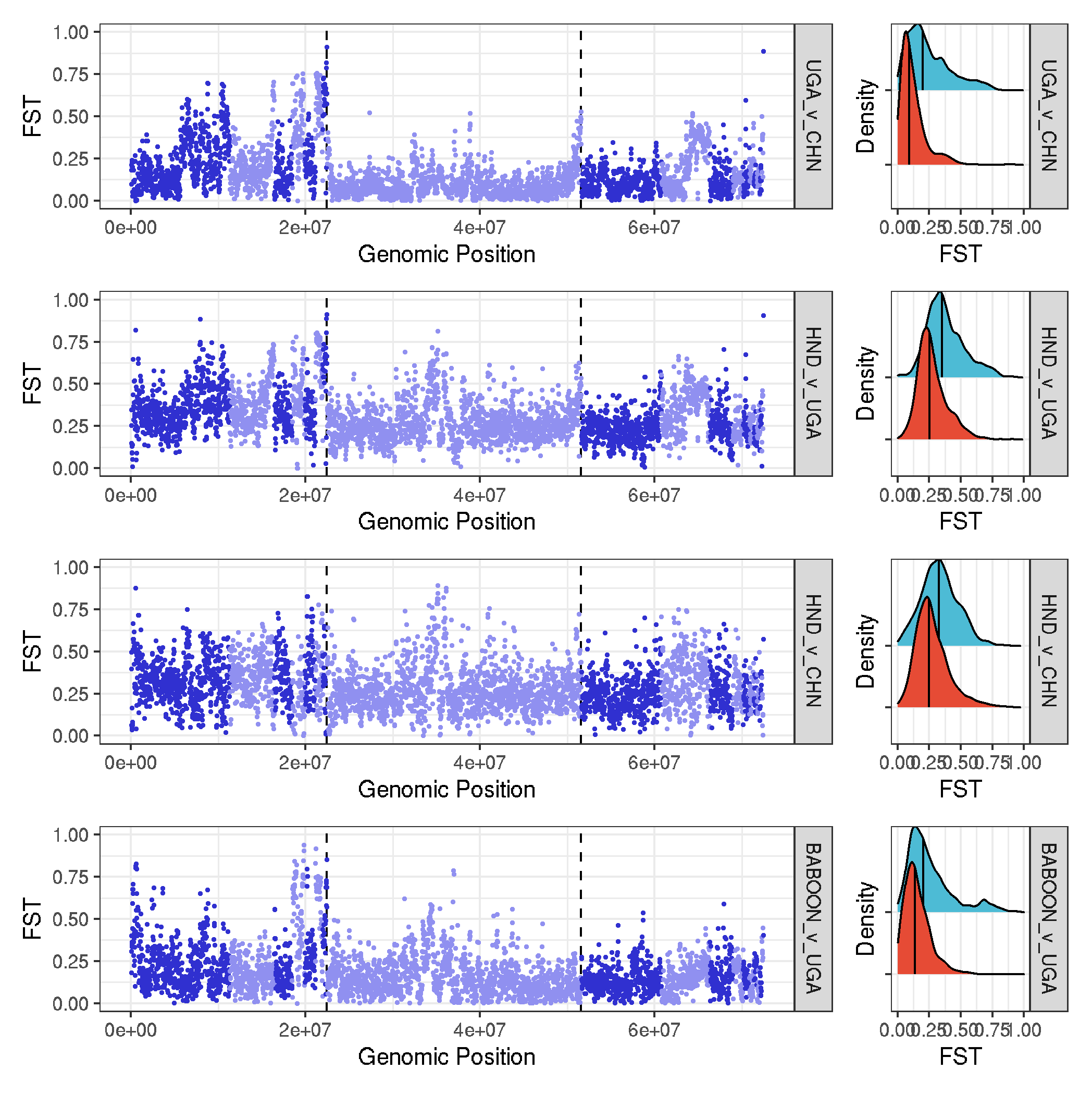
# using a function to allow me to put the facets in the order I want
#--- function
plot_gw_fst <- function(pair, type){

tmp_data <- data %>% filter(data_type==type & comparison==pair )

plot_gw <- ggplot(tmp_data, aes(position*20000, value, col=chromosome)) +
     geom_vline(xintercept=c(1122*20000,2580*20000), size=0.5, linetype="dashed")+
     geom_point(size=0.25) +
     scale_colour_cyclical(values = c("#3030D0", "#9090F0")) +
     facet_grid(comparison~.) +
     ylim(0,1) +
     theme_bw() +
     labs(x="Genomic Position", y="FST")

plot_density <- ggplot(tmp_data, aes(value, chr_type, fill=chr_type), guide="none") +
     geom_density_ridges(quantile_lines=TRUE, quantile_fun=function(x,...)median(x), size=0.5) +
     theme_bw() + theme(legend.position = "none", axis.text.y=element_blank()) +
     facet_grid(comparison~.) +
     xlim(0,1) +
     scale_fill_npg() +
     labs(x="FST", y="Density")

plot_gw + plot_density + plot_layout(widths = c(5, 1))

}



# make fst plots and assemble them
plot_UGA_v_CHN_fst <- plot_gw_fst("UGA_v_CHN", "Fst")
plot_HND_v_UGA_fst <- plot_gw_fst("HND_v_UGA", "Fst")
plot_HND_v_CHN_fst <- plot_gw_fst("HND_v_CHN", "Fst")
plot_BABOON_v_UGA_fst <- plot_gw_fst("BABOON_v_UGA", "Fst")

plot_UGA_v_CHN_fst / plot_HND_v_UGA_fst / plot_HND_v_CHN_fst / plot_BABOON_v_UGA_fst

ggsave("plots_genomewide_and_density_fst.pdf", width=7, height=6, useDingbats=FALSE)
ggsave("plots_genomewide_and_density_fst.png")


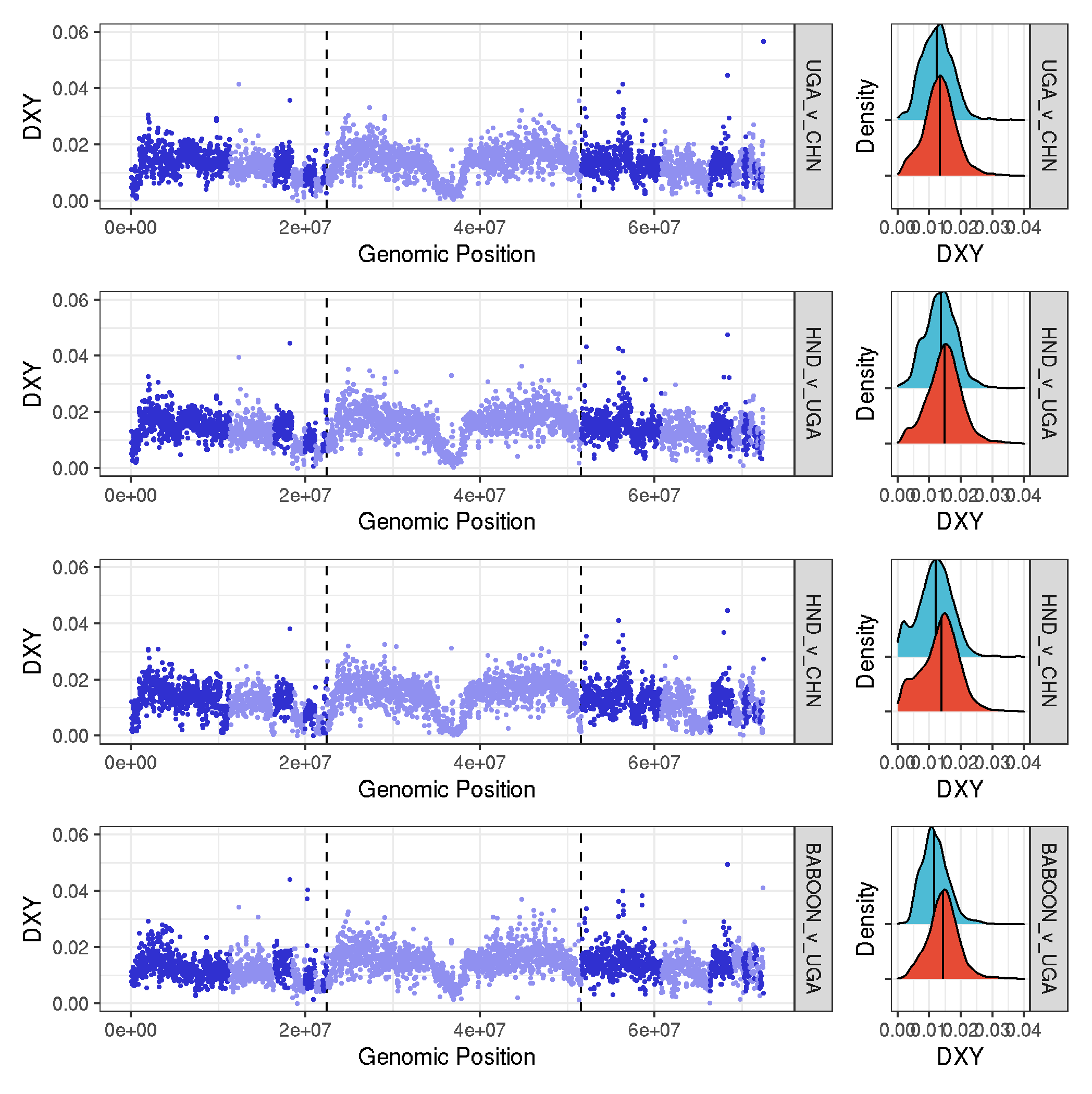
#--- function
plot_gw_dxy <- function(pair, type){

tmp_data <- data %>% filter(data_type==type & comparison==pair )

plot_gw <- ggplot(tmp_data, aes(position*20000, value, col=chromosome)) +
     geom_vline(xintercept=c(1122*20000,2580*20000), size=0.5, linetype="dashed")+
     geom_point(size=0.25) +
     scale_colour_cyclical(values = c("#3030D0", "#9090F0")) +
     facet_grid(comparison~.) +
     ylim(0,0.06) +
     theme_bw() +
     labs(x="Genomic Position", y="DXY")

plot_density <- ggplot(tmp_data, aes(value, chr_type, fill=chr_type), guide="none") +
     geom_density_ridges(quantile_lines=TRUE, quantile_fun=function(x,...)median(x), size=0.5) +
     theme_bw() + theme(legend.position = "none", axis.text.y=element_blank()) +
     facet_grid(comparison~.) +
     scale_fill_npg() +
     xlim(0,0.04) +
     labs(x="DXY", y="Density")


plot_gw + plot_density + plot_layout(widths = c(5, 1))

}



# make dxy plots and assemble them
plot_UGA_v_CHN_dxy <- plot_gw_dxy("UGA_v_CHN","Dxy")
plot_HND_v_UGA_dxy <- plot_gw_dxy("HND_v_UGA","Dxy")
plot_HND_v_CHN_dxy <- plot_gw_dxy("HND_v_CHN","Dxy")
plot_BABOON_v_UGA_dxy <- plot_gw_dxy("BABOON_v_UGA","Dxy")

plot_UGA_v_CHN_dxy / plot_HND_v_UGA_dxy / plot_HND_v_CHN_dxy / plot_BABOON_v_UGA_dxy

ggsave("plots_genomewide_and_density_dxy.pdf", width=7, height=6, useDingbats=FALSE)
ggsave("plots_genomewide_and_density_dxy.png")

• to go in the main text

• to go in the supplementary text

extracting top X% of Fst values for each comparison

library(tidyverse)

extract_top <- function(comparison, percent){
data <- read.table("trichuris_allsites_fst.txt", header=T)
data <- mutate(data, pairwise = paste(pop1, pop2, sep = '_v_'))

quantile <- (100-percent)/100

data_top_auto <- data %>%
     filter(chromosome!="Trichuris_trichiura_MITO") %>%
     filter(!str_detect(chromosome, "^Trichuris_trichiura_1")) %>%
     filter(!str_detect(chromosome, "^Trichuris_trichiura_00")) %>%
     filter(pairwise==comparison) %>%
     filter(avg_wc_fst > quantile(avg_wc_fst, quantile, na.rm=T)) %>%
     select(chromosome, window_pos_1, window_pos_2, avg_wc_fst)

data_top_sex <- data %>%
     filter(str_detect(chromosome, "^Trichuris_trichiura_1")) %>%
     filter(pairwise==comparison) %>%
     filter(avg_wc_fst > quantile(avg_wc_fst, quantile, na.rm=T)) %>%
     select(chromosome,window_pos_1,window_pos_2,avg_wc_fst)

data_top_other <- data %>%
     filter(chromosome!="Trichuris_trichiura_MITO") %>%
     filter(str_detect(chromosome, "^Trichuris_trichiura_00")) %>%
     filter(pairwise==comparison) %>%
     filter(avg_wc_fst > quantile(avg_wc_fst, quantile, na.rm=T)) %>%
     select(chromosome, window_pos_1, window_pos_2, avg_wc_fst)

data_top <- full_join(data_top_auto,data_top_sex)
data_top <- full_join(data_top,data_top_other)

write.table(data_top, file=paste0(comparison,".top_",percent,".coords"), row.names = F, col.names = F, quote = F, sep = '\t')
}

extract_top("HND_v_UGA", 5)
extract_top("UGA_v_CHN", 5)
extract_top("HND_v_CHN", 5)
extract_top("BABOON_v_UGA", 5)

# get the annotation
ln -s ../../01_REF/LIFTOFF/liftover_annotation.gff3

# extract the overlapping genes in the top X% datasets
for i in *top_?.coords; do
     bedtools intersect -b ${i} -a liftover_annotation.gff3 -wb |\
     awk '$3=="gene" {print $9}' | cut -f1 -d ";" | cut -f2 -d ":" \
     > ${i%.coords}.genes;
done

for i in *top_?.coords; do
     bedtools intersect -b ${i} -a liftover_annotation.gff3 -wb |\
     awk -F '[\t]' '$3=="gene" {print $10,$11,$12,$13,$4,$5,$9}' OFS="\t" | cut -f1 -d ";" | sed 's/ID=gene://g' \
     > ${i%.coords}.intersect;
done

# extract all gene IDs
cat liftover_annotation.gff3 |\
     awk '$3=="gene" {print $9}' |\
     cut -f1 -d ";" | cut -f2 -d ":" \
     > liftover_annotation.genelist

# use gProfiler to determine intersection
# gProfiler output
#     - UGA vs HND: https://biit.cs.ut.ee/gplink/l/qk_WBF0pSI
#     - UGA vs BABOON: https://biit.cs.ut.ee/gplink/l/5nu0UvV9T_

# extract gene ID information from top differentated genes
for FILE in *.top_5.genes; do
     while read GENE; do
          DATA=$(grep ${GENE} liftover_annotation.gff3 |\
          awk -F'[\t]' '{if($3=="gene") print $9}' |\
          grep -o "description=.*;" |\
          sed 's/;/\t/g' );\
          echo -e "${GENE}\t${DATA}";
     done < ${FILE} > ${FILE}_descriptions.txt;
done

Private and shared variation between populations

- testing correlation of Fst between UGA-CHN and UGA-Americas to see if there is variation shared by UGA-Americas that is not shared by UGA-China. If true, this might support independent migration into the Americas

```R
# load libraries
library(tidyverse)
library(patchwork)

uga_chn <- read.table("CHN_v_UGA_50k.windowed.weir.fst", header=T)
uga_chn$pair <- "UGAvCHN"
chn_americas <-read.table("CHN_v_AMERICAS_50k.windowed.weir.fst", header=T)
chn_americas$pair <- "CHNvAMERICAS"
uga_americas <-read.table("UGA_v_AMERICAS_50k.windowed.weir.fst", header=T)
uga_americas <- "UGAvAMERICAS"

data <- dplyr::bind_rows(uga_chn,chn_americas)
data <- dplyr::bind_rows(data,chn_americas)

uga_chn <- read.table("CHN_v_UGA_50k.windowed.weir.fst", header=T)
chn_americas <-read.table("CHN_v_AMERICAS_50k.windowed.weir.fst", header=T)
uga_americas <-read.table("UGA_v_AMERICAS_50k.windowed.weir.fst", header=T)

data <- dplyr::inner_join(uga_chn,chn_americas,by=c("CHROM","BIN_START"))
data <- dplyr::inner_join(data,uga_americas,by=c("CHROM","BIN_START"))
data <- data %>% select(CHROM,BIN_START,WEIGHTED_FST.x,WEIGHTED_FST.y,WEIGHTED_FST)
colnames(data) <- c("CHROM", "BIN_START", "FST_UGAvCHN", "FST_CHNvAMERICAS", "FST_UGAvAMERICAS")


plot_1 <-
     ggplot(data, aes(FST_UGAvCHN, FST_UGAvAMERICAS)) +
     geom_smooth(method = "lm", se = FALSE) +
     geom_point(size=0.5) +
     xlim(0,1) +
     ylim(0,1) +
     theme_bw()

plot_2 <-
     ggplot(data, aes(FST_UGAvCHN, FST_CHNvAMERICAS)) +
     geom_smooth(method = "lm", se = FALSE) +
     geom_point(size=0.5) +
     xlim(0,1) +
     ylim(0,1)+
     theme_bw()

plot_3 <-
     ggplot(data, aes(FST_UGAvAMERICAS, FST_CHNvAMERICAS)) +
     geom_smooth(method = "lm", se = FALSE) +
     geom_point(size=0.5) +
     xlim(0,1) +
     ylim(0,1)+
     theme_bw()

plot_1 + plot_2 + plot_3 + plot_layout(ncol=3)

cd /nfs/users/nfs_s/sd21/lustre118_link/trichuris_trichiura/04_VARIANTS/GATK_HC_MERGED

# extract data from UGA_CHN_AMERICAS samples, no missing data, to calculate per site allele freq, whcih will be used to calculate private and shared site frequencies
vcftools \
--gzvcf Trichuris_trichiura.cohort.nuclear_variants.final.recode.vcf.gz \
--max-missing 1 \
--keep UGA_x_nuclear_3x_animalPhonly.list \
--keep CHN_x_nuclear_3x_animalPhonly.list \
--keep AMERICAS_x_nuclear_3x_animalPhonly.list \
--recode \
--out UGA_CHN_AMERICAS

#> After filtering, kept 2430928 out of a possible 6571976 Sites


vcftools --vcf UGA_CHN_AMERICAS.recode.vcf --keep UGA_x_nuclear_3x_animalPhonly.list --freq --out UGA
vcftools --vcf UGA_CHN_AMERICAS.recode.vcf --keep CHN_x_nuclear_3x_animalPhonly.list --freq --out CHN
vcftools --vcf UGA_CHN_AMERICAS.recode.vcf --keep AMERICAS_x_nuclear_3x_animalPhonly.list --freq --out AMERICAS

paste UGA.frq CHN.frq AMERICAS.frq > UGA_CHN_AMERICAS.freq

# alt freq columns
#UGA_ALT = 8
#CHR_ALT = 16
#AMERICAS_ALT = 24

sed 's/:/\t/g' UGA_CHN_AMERICAS.freq | grep -v "CHROM" | cut -f8,16,24 > tmp; mv tmp UGA_CHN_AMERICAS.freq

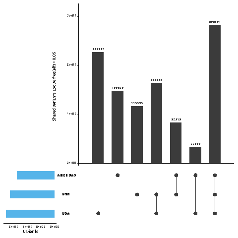
• make some plots, and summary data

# load libraries
library(tidyverse)
library(UpSetR)

data <- read.table("UGA_CHN_AMERICAS.freq",header=F)
colnames(data) <- c("UGA", "CHN", "AMERICAS")
data <- data %>% mutate_if(is.numeric, ~1 * (. > 0.05))

pdf(file="UGA_CHN_AMERICAS_shared_v_private_variants.pdf", onefile=FALSE)
upset(data,sets.bar.color = "#56B4E9", point.size = 3.5, mainbar.y.label = "Shared variants above freq(alt) = 0.05", sets.x.label = "Variants")
dev.off()

png(file="UGA_CHN_AMERICAS_shared_v_private_variants.png")
upset(data,sets.bar.color = "#56B4E9", point.size = 3.5, mainbar.y.label = "Shared variants above freq(alt) = 0.05", sets.x.label = "Variants")
dev.off()

data %>% group_by_all() %>% summarise(COUNT = n()) %>% mutate(freq = COUNT / sum(COUNT))

UGA	CHN	AMERICAS	COUNT	FREQ
0	0	0	1811631
0	0	1	148234
0	1	0	116536
0	1	1	83018
1	0	0	226805
1	0	1	33990
1	1	0	164206
1	1	1	282751

• note: 0,0,0 are positions in whihc the freq is very low in all populaitons. These variants are not used in calculating totals.

• private = (148234+116536+226805) / total = 46.57094947%
• shared by all three = 282751 / total = 26.7873316%
• shared by UGA and Americas, not China = 33990 / total = 3.220152718%

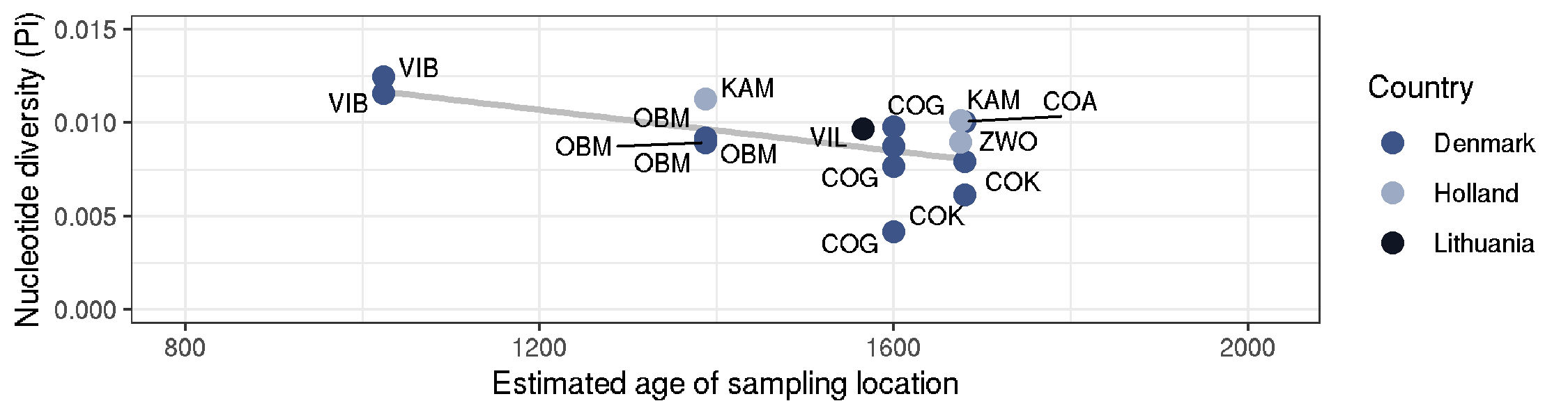
Ancient DNA - nucleotide diversity vs sampling age

# working directory
cd  ~/lustre118_link/trichuris_trichiura/05_ANALYSIS/POOLSEQ

library(tidyverse)
library(ggrepel)
library(patchwork)
library(ggsci)

data <- read.table("curated_data_npstats_age.txt", header=T)

country_colours <-
     c("Denmark" = "#3C5488",
     "Holland" = "#9DAAC4",
     "Lithuania" = "#0F1522")

ggplot(data) +
     geom_smooth(aes(Age,Pi), method = "lm", colour="grey") +
     geom_point(aes(Age, Pi, colour = Country), size=3) +
     geom_text_repel(aes(Age, Pi, label=Population), size=3) +
     ylim(0,0.015) + xlim(800,2020) +
     theme_bw() + labs(x="Estimated age of sampling location", y="Nucleotide diversity (Pi)") +
     scale_colour_manual(values = country_colours)

ggsave("ancient_sites_Pi_over_time.png", height=2, width=7.5)
ggsave("ancient_sites_Pi_over_time.pdf", height=2, width=7.5, useDingbats=FALSE)



ggplot(data2) +
     geom_smooth(aes(Age,Pi), method = "lm", colour="grey") +
     geom_point(aes(Age, Pi, colour = Country), size=3) +
     geom_text_repel(aes(Age, Pi, label=Population), size=3) +
     ylim(0,0.015) + xlim(800,2020) +
     theme_bw() + labs(x="Estimated age of sampling location", y="Nucleotide diversity (Pi)") +
     scale_colour_manual(values = country_colours)

Figure: map

• new main text figure

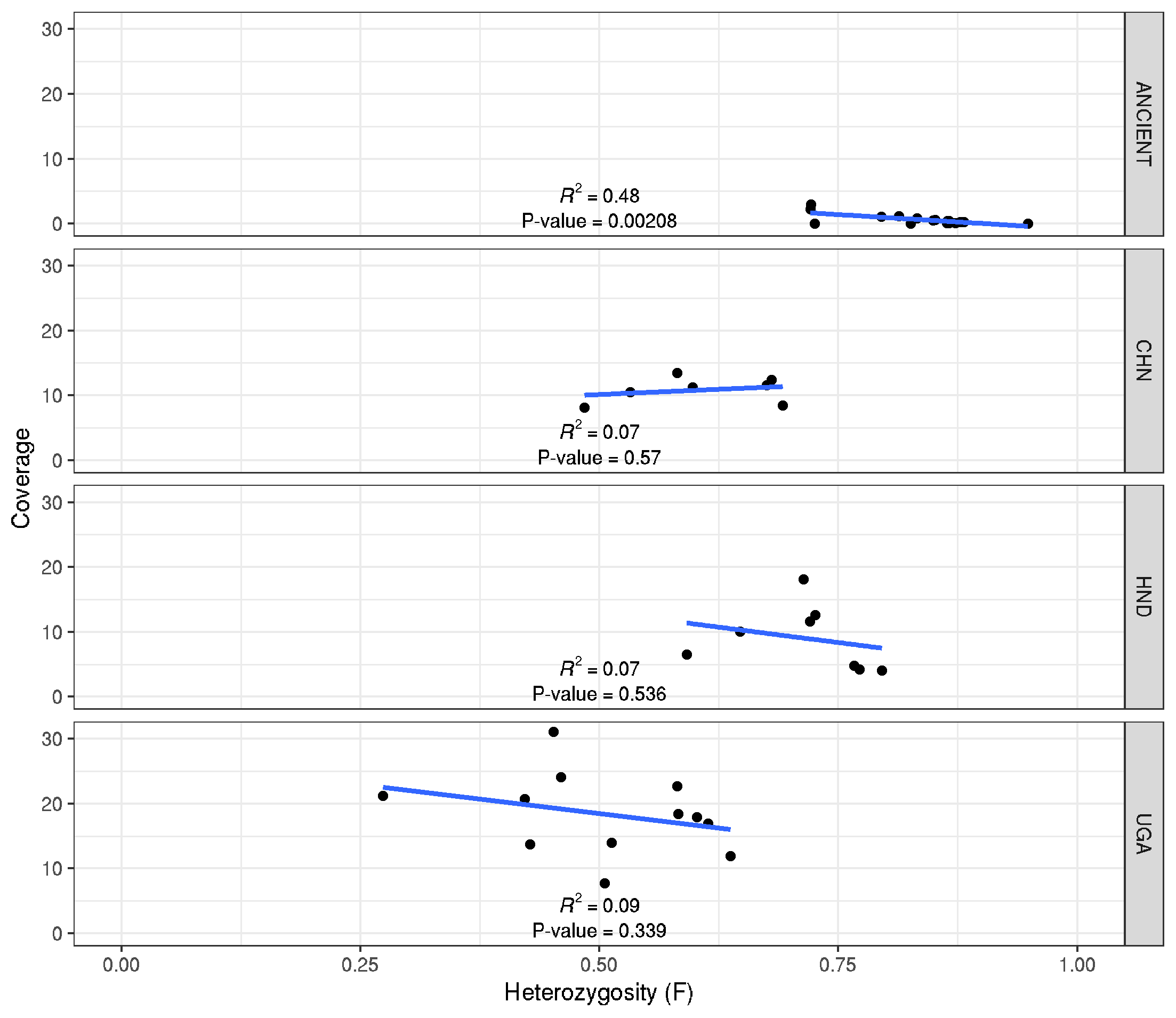
Sample Heterozygosity vs sequencing coverage

library(tidyverse)
library(ggpmisc)

data <- read.table("heterozygosity_x_coverage.txt", header = T)

formula <- x ~ y

ggplot(data,aes(F,COV)) +
     geom_point() + xlim(0,1) +
     labs(x="Heterozygosity (F)", y="Coverage") +
     facet_grid(POPULATION~.) + theme_bw() +
     geom_smooth(method = "lm", se = FALSE)+
     stat_fit_glance(method = 'lm',
          method.args = list(formula = formula),
          geom = 'text',
          aes(label = paste("P-value = ", signif(..p.value.., digits = 3), sep = "")),
          label.x = 0.5, label.y = 0.5, size = 3) +
     stat_poly_eq(aes(label = paste(..rr.label..)),
          label.x = 0.5, label.y = 0.15, formula = formula, parse = TRUE, size = 3)

ggsave("heterozygosity_x_coverage.png")
ggsave("heterozygosity_x_coverage.pdf", height=7, width=7, useDingbats=FALSE)

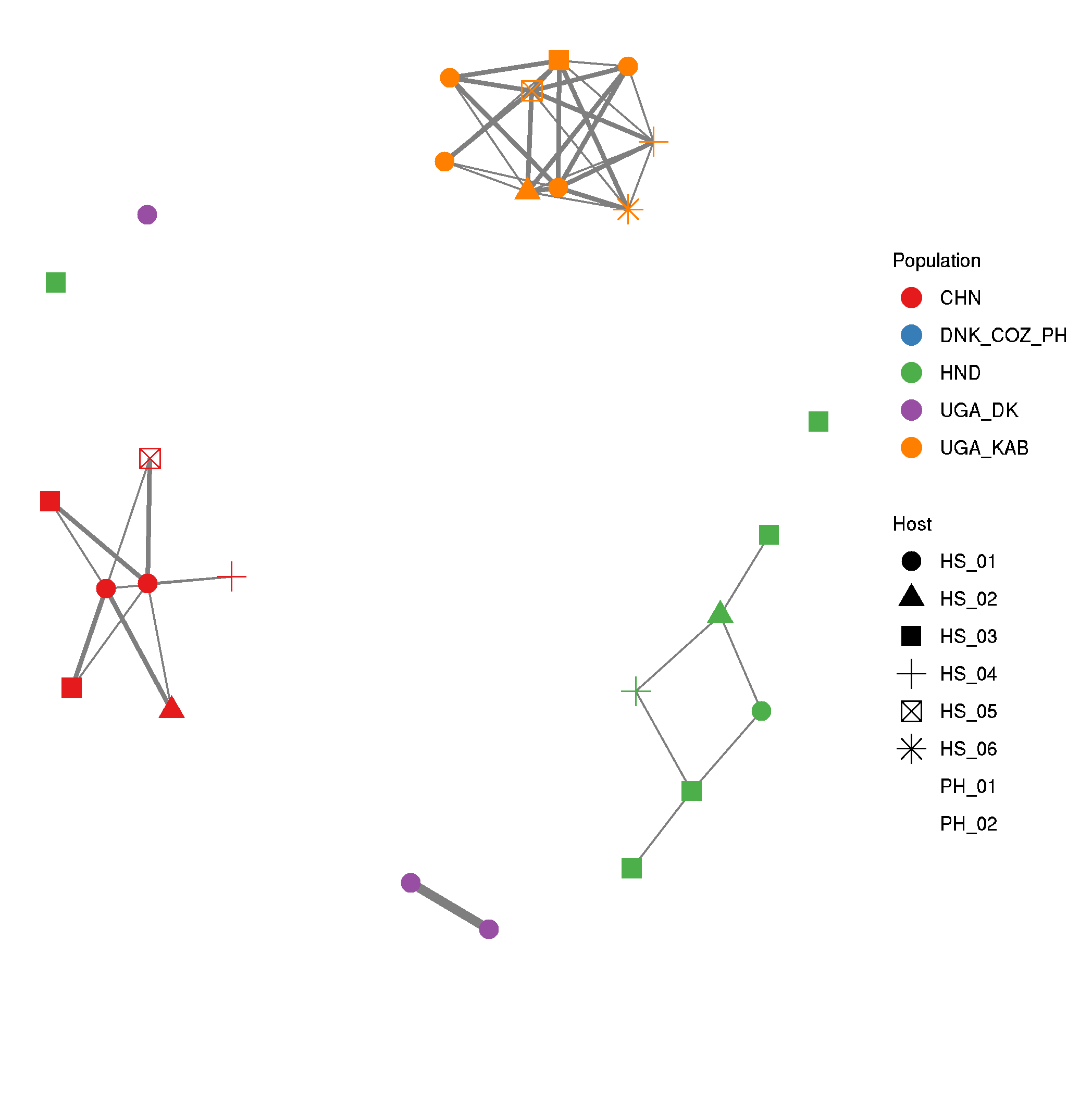
Relatedness and kinship between samples in a population

• Want to know to what degree individual worms from a population are related to each other.
• can do this via calculating kinship coefficients, to determine 1st, 2nd, 3rd degree relatives

# run vcftools to calculated relatedness
vcftools --gzvcf nuclear_samples3x_missing0.8_animalPhonly.recode.vcf.gz --relatedness2 --max-missing 1

# extract relevant pairwise comparisons for making the network.
#--- note only want within population comparisons, rather than between populations
#--- also want to remove self v self.
>allpops.relatedness2
for i in CHN DNK_COZ_PH HND UGA_DK UGA_KAB ; do
     awk -v name=$i '$1~name && $2~name {print $0,name}' OFS="\t" out.relatedness2 |\
     awk '{if($1!=$2) print $8,$1,$2,$7}' OFS="\t" >> allpops.relatedness2;
done

# make a file with population groups for colouring the network in
cut -f 1,2 allpops.relatedness2 | sort | uniq > metadata.txt

# load libraries
# https://briatte.github.io/ggnet/
library(tidyverse)
library(GGally)
library(network)
library(sna)
library(ggplot2)


# read data
data <- read.table("allpops.relatedness2")
metadata <- read.table("metadata.txt")


# convert kinship coefficients into a coded 1st, 2nd, 3rd degree relatives
data_1 <-
     data %>%
     mutate(V4 = if_else(V4 >= 0.05 & V4 < 0.10125, 0.5,
               if_else(V4 >= 0.10125 & V4 < 0.1925, 1,
               if_else(V4 >= 0.1925 & V4 < 0.375, 2, 0))))

# coding:
#0 degree = 0.5
#1st degree = 0.25 (0.1925-0.375)
#2nd degree = 0.125 (0.10125-0.1925)
#3rd degree = 0.0675 (0.05-0.10125)
#4th degree = 0.03375

# convert data from paired observations to a matrix of observations
data_2 <-
     data_1 %>%
     unique() %>%
     pivot_wider(., id_cols=V2, names_from=V3, values_from=V4, values_fill=0)

data_3 <- as.data.frame(data_2, row.names=F)

# clean up matrix
data_4 <-
     data_3 %>%
     remove_rownames %>%
     column_to_rownames(var="V2")

data_4.1 <- as.matrix(data_4)

# make the network
data_5 <- network(data_4.1, ignore.eval = FALSE, names.eval = "kinship")

# add the population metaddata
data_5 %v% "Population" = metadata$V1
data_5 %v% "Host" = metadata$V3

# set colours for populations
col =  c("CHN" = "#E64B35B2", "DNK_COZ_PH" = "#00A087B2", "HND" = "#8491B4B2", "NLD" = "#91D1C2B2", "UGA_KAB" = "#DC0000B2", "UGA_DK" = "#DC0000B8")

col <-
     c("CHN" = "#00A087",
     "CMR" = "#902F21",
     "DNK" = "#3C5488",
     "ESP" = "#E7EAF0",
     "HND" = "#4DBBD5",
     "NLD" = "#9DAAC4",
     "UGA" = "#E64B35",
     "LTU" = "#0F1522",
     "TZA" = "#F2A59A")


#set.edge.attribute(data_5, "lty", ifelse(data_5 %e% "kinship" = 3, 1, ifelse(data_5 %e% "kinship" = 2, 2, 3)))

# plot the network
ggnet2(data_5, edge.size = "kinship", color = "Population", palette = "Set1", size=4, shape="Host")

# save it
ggsave("kinship_network.pdf", useDingbats=F, height=8, width=8)
ggsave("kinship_network.png")

genome-wide analyses presented in the original draft of the manuscript, but subsequently improved upon

Nucleotide diversity and Tajima’s D

# extract scaffolds in chromosome linkage groups
#- this represents 72375426 of 80573711, or 89.83% of genome
cat ../../01_REF/trichuris_trichiura.fa.fai | grep -v "Trichuris_trichiura_00_*" | grep -v "MITO" | awk '{print $1,1,$2}' OFS="\t" > chromosome_scaffolds.bed

# extract nucleotide diversity for each group
for i in ancient_x_nuclear_3x_animalPhonly.list \
     CHN_x_nuclear_3x_animalPhonly.list \
     BABOON_x_nuclear_3x_animalPhonly.list \
     HND_x_nuclear_3x_animalPhonly.list \
     UGA_x_nuclear_3x_animalPhonly.list; do \
          vcftools --gzvcf nuclear_samples3x_missing0.8_animalPhonly.recode.vcf.gz --keep ${i} --bed chromosome_scaffolds.bed --window-pi 50000 --out ${i%.list}_50k;
          vcftools --gzvcf nuclear_samples3x_missing0.8_animalPhonly.recode.vcf.gz --keep ${i} --bed chromosome_scaffolds.bed --TajimaD 50000 --out ${i%.list}_50k;
     done

# summary stats for Pi
for i in *_50k.windowed.pi;
     do echo ${i}; cat ${i} | datamash --headers mean 5 sstdev 5;
done

# summary stats for TajD
for i in *_50k.Tajima.D;
     do echo ${i}; cat ${i} | datamash --headers mean 4 sstdev 4 --narm;
done

_50k.Tajima.D

# other random vcftools analyses
vcftools --gzvcf nuclear_samples3x_missing0.8_animalPhonly.recode.vcf.gz --indv-freq-burden --out nuclear_samples3x_missing0.8_animalPhonly

vcftools --gzvcf nuclear_samples3x_missing0.8_animalPhonly.recode.vcf.gz --het --out nuclear_samples3x_missing0.8_animalPhonly

vcftools --gzvcf nuclear_samples3x_missing0.8_animalPhonly.recode.vcf.gz --relatedness --out nuclear_samples3x_missing0.8_animalPhonly

vcftools --gzvcf nuclear_samples3x_missing0.8_animalPhonly.recode.vcf.gz --FILTER-summary --out nuclear_samples3x_missing0.8_animalPhonly

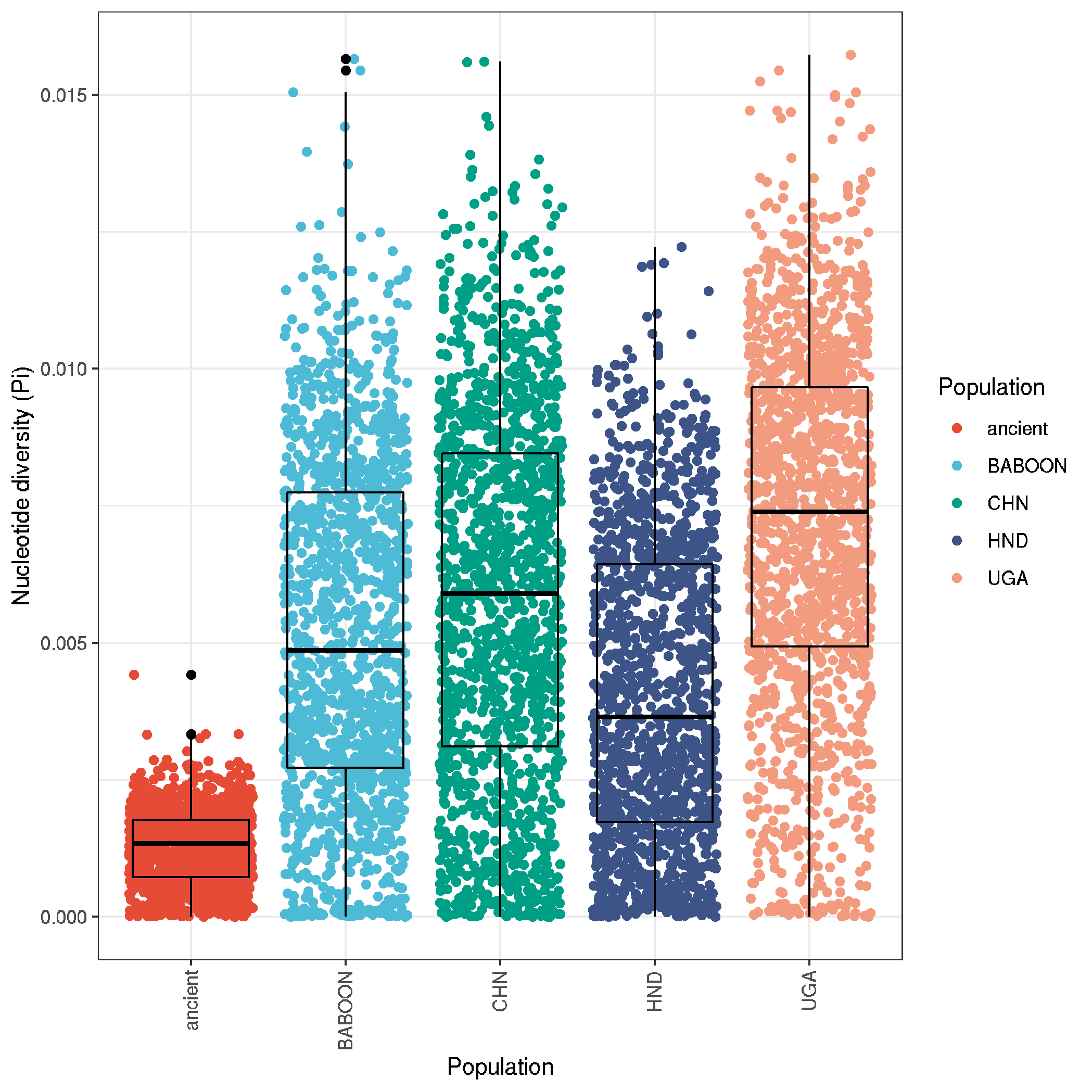
plot nucleotide diversities

# load libraries
library(tidyverse)
library(ggsci)

# list file names
file_names <- list.files(path = "./",pattern = "_x_nuclear_3x_animalPhonly_50k.windowed.pi")

# load data using file names, and make a formatted data frame
data <-
     purrr::map_df(file_names, function(x) {
	data <- read.delim(x, header = T, sep="\t")
     data <- tibble::rowid_to_column(data, "NUM")
	cbind(pop_id = gsub("_x_nuclear_3x_animalPhonly_50k.windowed.pi","",x), data)
	})

ggplot(data,aes(pop_id,PI,col=pop_id)) +
     geom_jitter() +
     geom_boxplot(fill=NA, col="black") +
     labs(x = "Population" , y = "Nucleotide diversity (Pi)", colour = "Population") +
     theme_bw() +
     theme(axis.text.x = element_text(angle = 90, vjust = 0.5, hjust=1)) +
     scale_color_npg()

ggsave("plot_nucleotide_diversity_boxplot.png")
ggsave("plot_nucleotide_diversity_boxplot.pdf", useDingbats=F, height=5, width=5)


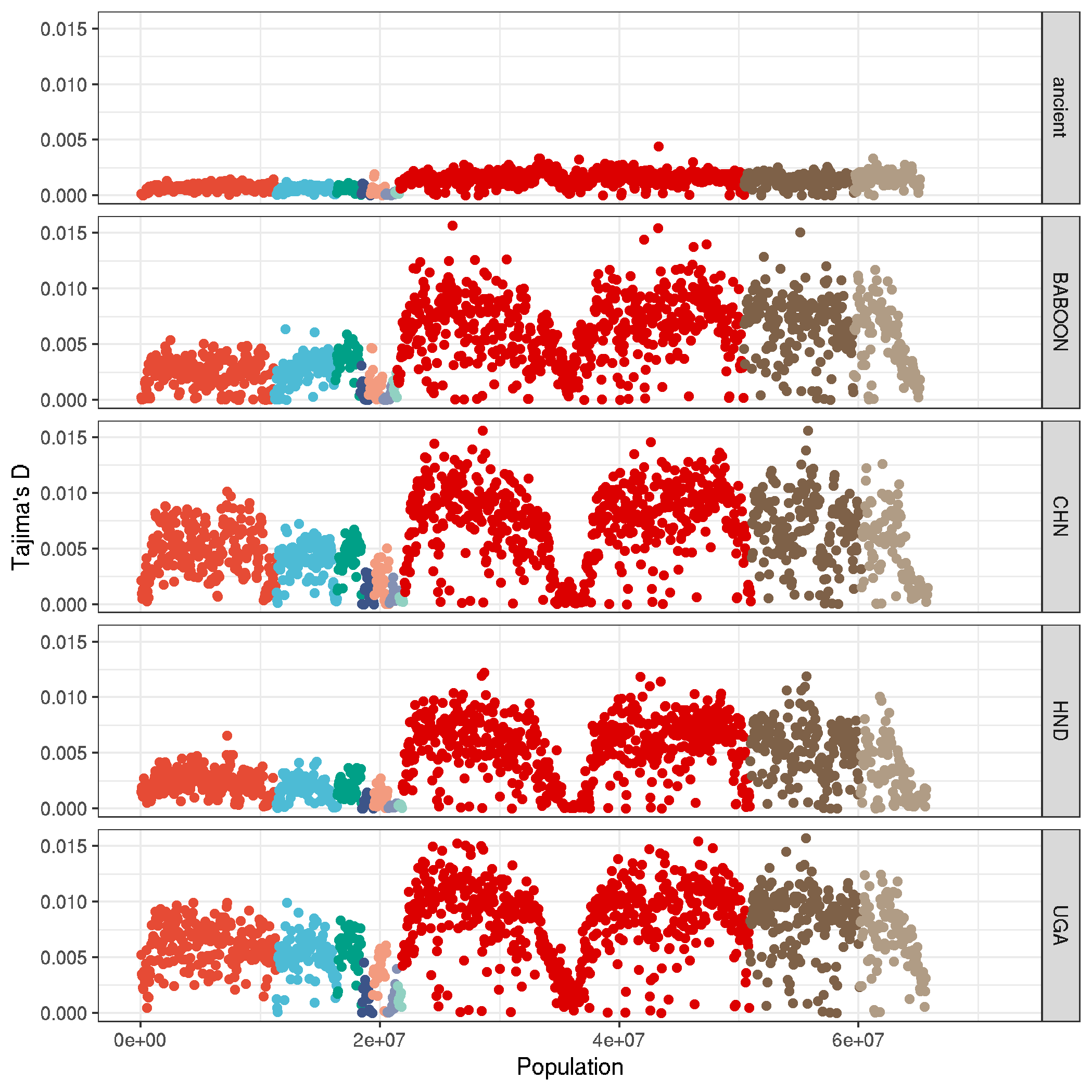
ggplot(data,aes(NUM*50000,PI,col=CHROM, group=pop_id)) +
     geom_point() +
     labs(x = "Population" , y = "Nucleotide diversity (Pi)", col=NA) +
     theme_bw() +
     facet_grid(pop_id~.) +
     theme(legend.position = "none")


ggplot(data,aes(NUM*50000,PI,col=CHROM, group=pop_id)) +
     geom_point() +
     labs(x = "Population" , y = "Tajima's D", col=NA) +
     theme_bw() +
     facet_grid(pop_id~.) +
     theme(legend.position = "none") +
     scale_color_npg()

ggsave("plot_nucleotide_diversity_genomewide.png")

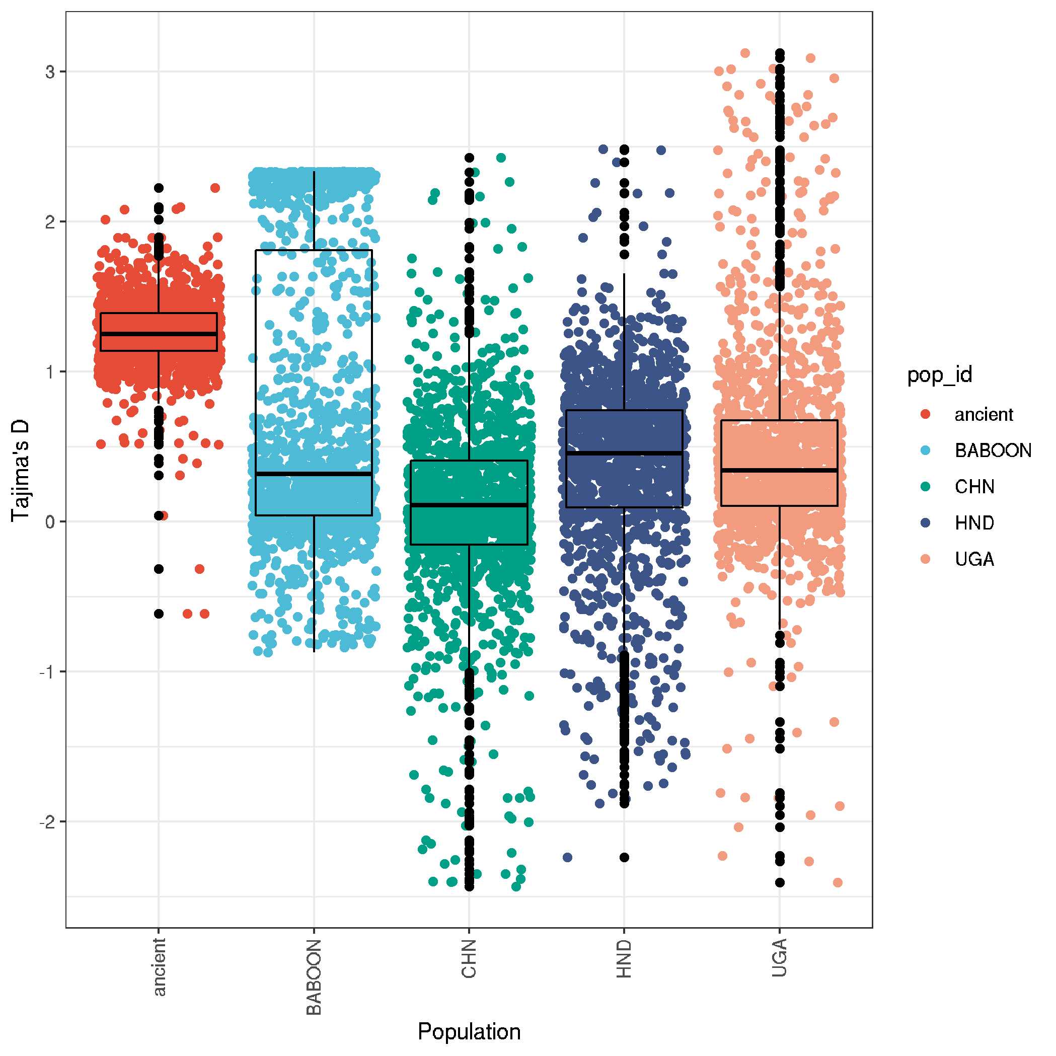
plot Tajimas D

library(tidyverse)
library(ggsci)

# list file names
file_names <- list.files(path = "./",pattern = "_x_nuclear_3x_animalPhonly_50k.Tajima.D")

# load data using file names, and make a formatted data frame
data <-
     purrr::map_df(file_names, function(x) {
	data <- read.delim(x, header = T, sep="\t")
     data <- tibble::rowid_to_column(data, "NUM")
	cbind(pop_id = gsub("_x_nuclear_3x_animalPhonly_50k.Tajima.D","",x), data)
	})

# plot boxplots and distributions of Tajima's D
ggplot(data,aes(pop_id,TajimaD,col=pop_id)) +
     geom_jitter() +
     geom_boxplot(fill=NA, col="black") +
     labs(x = "Population" , y = "Tajima's D") +
     theme_bw() +
     theme(axis.text.x = element_text(angle = 90, vjust = 0.5, hjust=1)) +
     scale_color_npg()

ggsave("plot_tajimaD_boxplot.png")
ggsave("plot_tajimaD_boxplot.pdf", useDingbats=F, width=8, height=5)


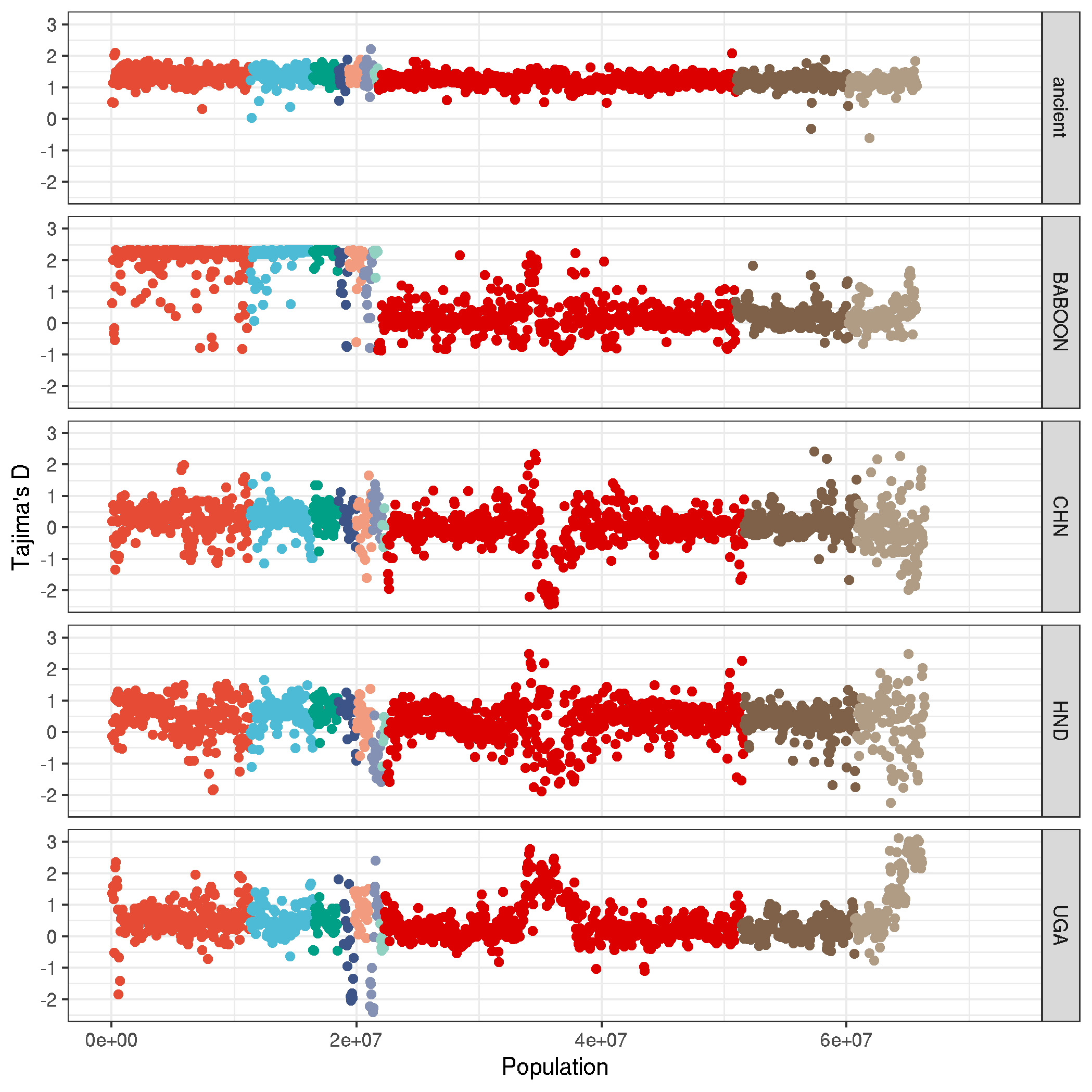
ggplot(data,aes(NUM*50000,TajimaD,col=CHROM, group=pop_id)) +
     geom_point() +
     labs(x = "Population" , y = "Tajima's D", col=NA) +
     theme_bw() +
     facet_grid(pop_id~.) +
     theme(legend.position = "none") +
     scale_color_npg()

ggsave("plot_tajimaD_genomewide.png")
ggsave("plot_tajimaD_genomewide.pdf", useDingbats=F, width=7, height=7)


plot_tajD <-
     ggplot(data,aes(NUM*50000,TajimaD,col=pop_id, group=pop_id)) +
     geom_smooth(span = 0.1, se = FALSE) +
     labs(x = "Population" , y = "Tajima's D", col= "Population") +
     theme_bw() +
     theme() +
     scale_color_npg()

plot_Pi + plot_tajD + plot_layout(ncol = 1, guides = "collect")

Genome wide genetic differentiation

# run vcftools weir-fst-pop for all pairwise combinations of populatiions
for i in ancient_x_nuclear_3x_animalPhonly.list \
BABOON_x_nuclear_3x_animalPhonly.list \
CHN_x_nuclear_3x_animalPhonly.list \
HND_x_nuclear_3x_animalPhonly.list \
UGA_x_nuclear_3x_animalPhonly.list; do \
     for j in ancient_x_nuclear_3x_animalPhonly.list \
     BABOON_x_nuclear_3x_animalPhonly.list \
     CHN_x_nuclear_3x_animalPhonly.list \
     HND_x_nuclear_3x_animalPhonly.list \
     UGA_x_nuclear_3x_animalPhonly.list; do \
          if [[ "$i" == "$j" ]] || [[ -f ${i%_x_nuclear_3x_animalPhonly.list}_v_${j%_x_nuclear_3x_animalPhonly.list}_50k.windowed.weir.fst ]] || [[ -f ${j%_x_nuclear_3x_animalPhonly.list}_v_${i%_x_nuclear_3x_animalPhonly.list}_50k.windowed.weir.fst ]]; then
               echo "Same, same, move on"
               else
               vcftools --gzvcf nuclear_samples3x_missing0.8_animalPhonly.recode.vcf.gz --bed chromosome_scaffolds.bed --weir-fst-pop ${i} --weir-fst-pop ${j} --fst-window-size 50000 --out ${i%_x_nuclear_3x_animalPhonly.list}_v_${j%_x_nuclear_3x_animalPhonly.list}_50k;
          fi;
     done;
done

• make some plots

# load libraries
library(tidyverse)
library(ggsci)
library(patchwork)

# list file names
file_names <- list.files(path = "./",pattern = "_50k.windowed.weir.fst")

# load data using file names, and make a formatted data frame
data <-
     purrr::map_df(file_names, function(x) {
	data <- read.delim(x, header = T, sep="\t")
     data <- tibble::rowid_to_column(data, "NUM")
	cbind(sample_pair = gsub("_50k.windowed.weir.fst","",x), data)
	})

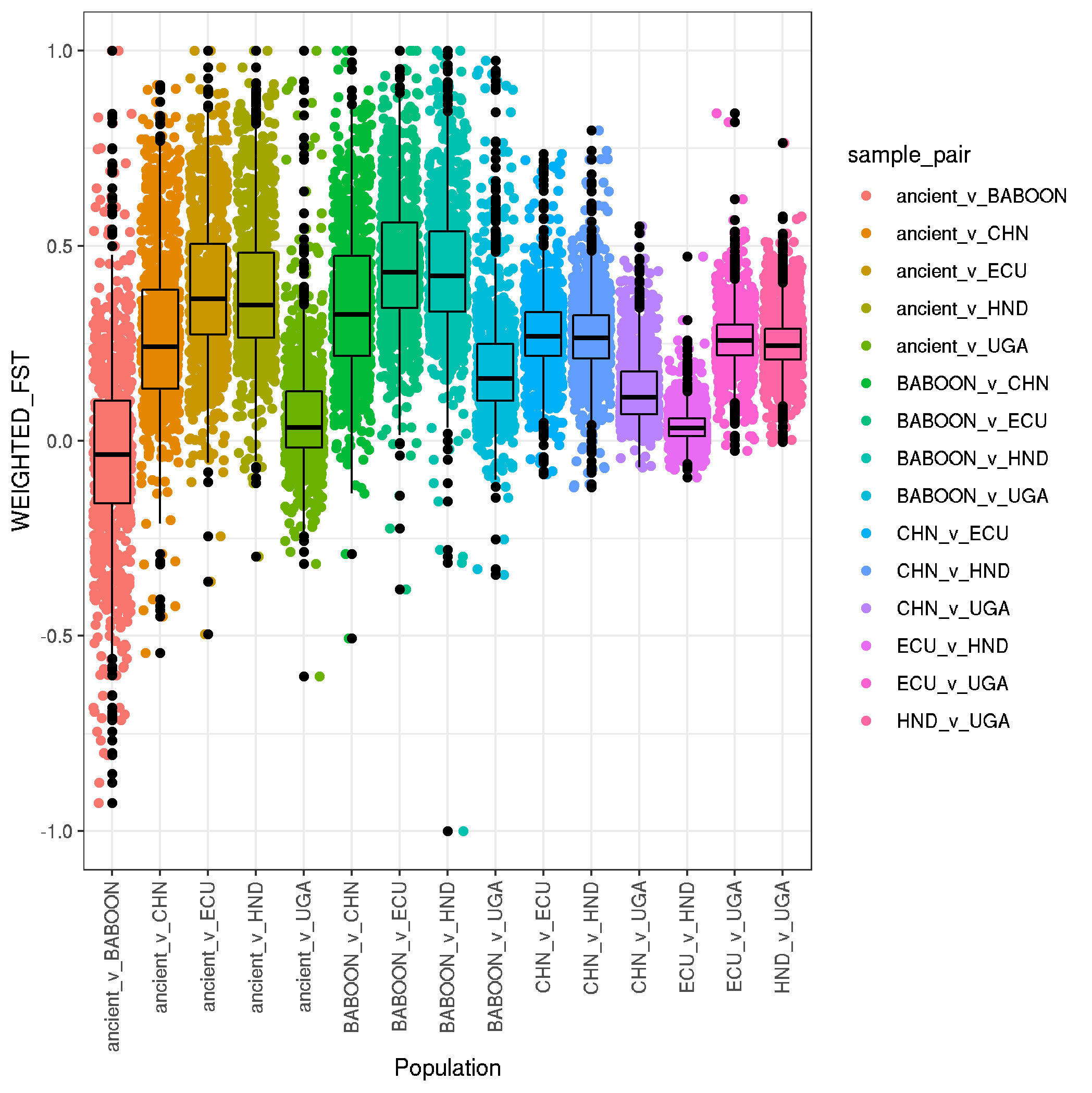
# plot boxplots and distributions of pairwise Fst analyses
ggplot(data,aes(sample_pair,WEIGHTED_FST,col=sample_pair)) +
     geom_jitter() +
     geom_boxplot(fill=NA, col="black") +
     labs(x = "Population" , y = "WEIGHTED_FST") +
     theme_bw() +
     theme(axis.text.x = element_text(angle = 90, vjust = 0.5, hjust=1))

# save it
ggsave("plot_human_pop_pairwise_FST_boxplot.png")


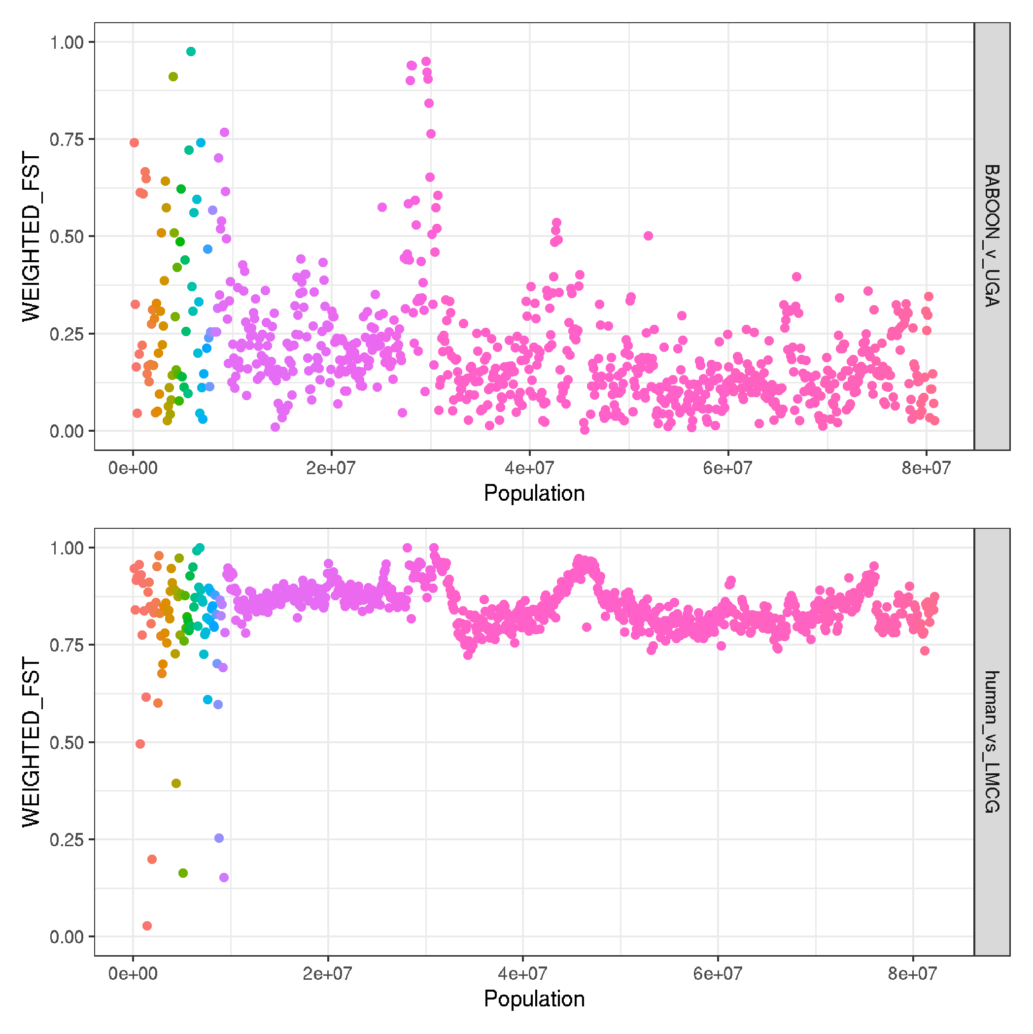
# plot genome-wide distributions of pairwise Fst analyses
ggplot(data, aes(NUM*50000, WEIGHTED_FST, col=CHROM, group=sample_pair)) +
     geom_point() +
     labs(x = "Population" , y = "WEIGHTED_FST", col=NA) +
     theme_bw() +
     facet_grid(sample_pair~.) +
     theme(legend.position = "none") +
     scale_color_npg()

ggsave("plot_human_pop_pairwise_FST__genomewide.png")


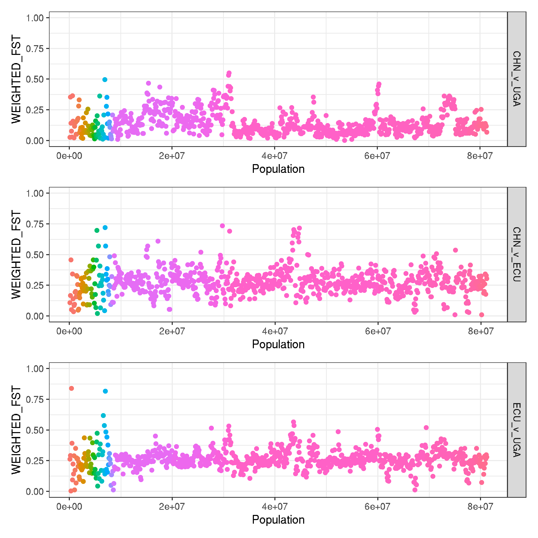
# function to load specific datasets to make multipanel figures
plot_pairwise_fst <- function(file) {
     # load and prep data
     data <- read.delim(file, header=T, sep="\t")
     data <- tibble::rowid_to_column(data, "NUM")
     data$COMPARISON <- gsub("_50k.windowed.weir.fst","",file)
     # plot
     ggplot(data, aes(NUM*50000, WEIGHTED_FST, col=CHROM)) +
     geom_point(size=0.5) +
     labs(x = "Genomic position (bp)" , y = "Weighted FST", col=NA) +
     theme_bw() + ylim(0,1) +
     facet_grid(COMPARISON~.) +
     theme(legend.position = "none", text = element_text(size = 10))+
     scale_color_npg()
}

# for main text
CHN_v_UGA_fst <- plot_pairwise_fst("CHN_v_UGA_50k.windowed.weir.fst")
HND_v_UGA <- plot_pairwise_fst("HND_v_UGA_50k.windowed.weir.fst")
CHN_v_HND <- plot_pairwise_fst("CHN_v_HND_50k.windowed.weir.fst")
BABOON_v_UGA_fst <- plot_pairwise_fst("BABOON_v_UGA_50k.windowed.weir.fst")

CHN_v_UGA_fst + HND_v_UGA + CHN_v_HND + BABOON_v_UGA_fst + plot_layout(ncol=1)

ggsave("plot_pairwise_FST_genomewide.pdf", width=170, height=150, units="mm")

# BABOON_v_UGA_fst <- plot_pairwise_fst("BABOON_v_UGA_50k.windowed.weir.fst")
# human_vs_LMCG_fst <- plot_pairwise_fst("human_vs_LMCG_50k.windowed.weir.fst")
#
# BABOON_v_UGA_fst + human_vs_LMCG_fst + plot_layout(ncol=1)
# ggsave("plot_humananimal_pop_pairwise_FST_genomewide.png")
#
# # for supplementary data
# CHN_v_UGA_fst <- plot_pairwise_fst("CHN_v_UGA_50k.windowed.weir.fst")
#
# CHN_v_UGA_fst + CHN_v_ECU_fst + ECU_v_UGA_fst + plot_layout(ncol=1)
# ggsave("plot_human_pop_pairwise_FST_genomewide.png")
#

• boxplot summaries

• genomewide - human populations

• genomewide - human v animal populations